Cours 6 - Calculs numériques

Rappels

Un ordinateur n’est au final qu’une grosse calculatrice avec plusieurs avantages:

Meilleur clavier
Meilleur écran
Plus de puissance

Il est extrêmement commun pour un ingénieur d’utiliser un ordinateur pour effectuer des calculs. L’utilisation de Python dans ce domaine est très répandue dans le monde professionnel.

Rappels: Calcul numérique

Différent du calcul symbolique
Méthodes de résolution itératives Série de valeurs qui s’approchent de la solution
Solution numérique approchée Souvent aussi proche que l’on veut

Outil: `numpy`

Bibliothèque à installer

> python -m pip install numpy
Permet de travailler très efficacement avec des vecteurs de nombres
Incontournable pour le calcul numérique en Python

`numpy`

Utilisation d’un alias pour l’import
```
import numpy as np
```
Création d’un vecteur
```
v = np.array([1, 1, 3])
```

Opérations

print(2*v)                   # Multiplication par un scalaire
print(v+v)                   # Somme
print(v.dot(v))              # Produit scalaire
print(v @ v)                 # Produit scalaire
v2 = np.array([2, -1, 2]
print(np.cross(v, v2)))      # Produit vectoriel
print(np.linalg.norm(v))     # Norme

Vecteurs

Plusieurs manières de créer des vecteurs de valeurs Depuis une structure Python, ou par des fonctions de Numpy

np.array([1, 2, 3])
np.zeros(5)
np.ones(10)
np.random.random(10)
np.random.randn(10)
np.linspace(0, 10, 5)
np.arange(0, 10, 0.2)

Opérations

Entre vecteur et scalaire

a = np.array([1, 2, 3, 4])
a + 1       # [2, 3, 4, 5]
2 * a       # [2, 4, 6, 8]
a ** 2      # [1, 4, 9, 16]
1 / a       # [1.0, 0.5, 0.3333, 0.25]
a < 3    # [True, True, False, False]

Entre vecteurs de même taille élément par élément

a = np.array([1, 2, 3, 4])
b = np.array([5, 6, 7, 8])
a + b    # [6, 8, 10, 12]
a * b    # [5, 12, 21, 32]

Fonctions vectorisées

Fonctions qui s’applique sur tous les éléments d’un vecteur

x = np.array([1, 2, 3])

# Fonction standard ne marche pas
y = math.sin(x) # Error

# Fonction vectorisée existe dans numpy
y = np.sin(x)

Créer une fonction vectorisée

La plupart des opérations de base sont déjà supportées par numpy.
Mais il est facile de créer des fonctions vectorisées:

@np.vectorize
def fun(a, b):
  if a > b:
    return 1
  return -1

x = np.array([1, 2, 3])
y = np.array([3, 2, 1])

print(fun(x, y))

`numpy`: Calcul Matriciel

numpy permet aussi de travailler avec des matrices

A = np.array([[1, 2],
              [3, 4]])

Même opérations que le vecteurs

Opérations avec scalaires

A = np.array([[1, 2],
              [3, 4]])
2*A         #[[2, 4],
            # [6, 8]]

Opérations avec tableaux de même taille et produit matriciel

B = np.array([[5, 6], [7, 8]])
A * B       # produit élément par élément
A @ B       # produit matriciel

Fonctions sur les tableaux

np.sin(A)   # [[ 0.84147098  0.90929743]
            #  [ 0.14112001 -0.7568025 ]]

Attributs

x = np.array([[1, 2],
              [3, 4],
              [5, 6]])

x.ndim   # Dimension => 2
x.shape  # Forme => (3, 2)
x.size   # Nombre total d’éléments => 6
x.dtype  # Type de données stockées => dtype('int32')

Indexation

x = np.array([[1, 2],
              [3, 4],
              [5, 6]])

x[0, 1]                 # x[0][1] => 2

# Slice
x[:2, 1]                # [2, 4]
x[[0, 2], :]            # [[1, 2], [5, 6]]

# Indexation booléenne
x[[[True , False],
   [False, True ],
   [True , True ]]]     # [1, 4, 5, 6]
x[x < 4]                # [1, 2, 3]

# Edition conditionnelle
x[x < 4] = 0            # [[0, 0],
                        #  [0, 4],
                        #  [5, 6]]

Méthodes

x = np.array([[1, 2],
              [3, 4],
              [5, 6]])
x.reshape((2, 3))  # [[1, 2, 3],
                   #  [4, 5, 6]]

x.flatten()        # [1, 2, 3, 4, 5, 6]
x.diagonal()       # [1, 4]
x.trace()          # 5
x.sum(axis=1)      # [3, 7, 11]
y = x.transpose()  # [[1, 3, 5],
                   #  [2, 4, 6]]

Graphiques de fonctions

Utilisation du module matplotlib à installer

> python -m pip install matplotlib

Fonctionne en tandem avec numpy

Créer un graphique

Importer matplotlib
```
from matplotlib import pyplot as plt
```
Importer numpy
```
import numpy as np
```

Créer les abscisses des échantillons

# 100 valeurs entre -2 et 2
x = np.linspace(-5, 5, 100)

Calculer les ordonnées

# np.sin est la version vectorisée de sin
y = np.sin(x)

Dessiner le graphique
```
plt.figure()
plt.plot(x, y)
plt.show()
```

Graphique matplotlib — Graphique `matplotlib`

Style

Toutes les parties du graphique sont paramètrables

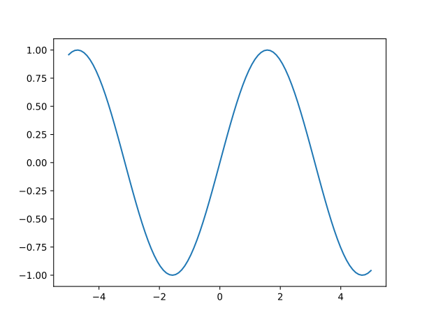
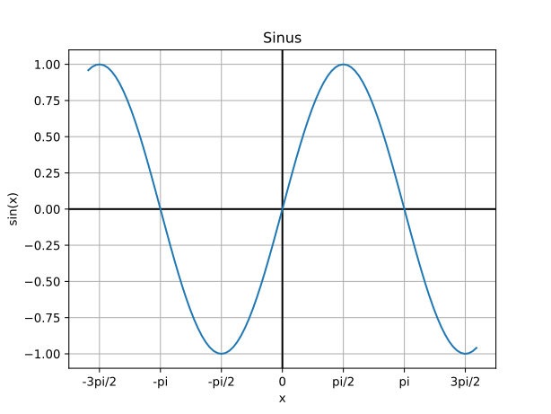
from matplotlib import pyplot as plt
import numpy as np

x = np.linspace(-5, 5, 100)
y = np.sin(x)
plt.figure()
plt.title("Sinus")              # Donne un titre à la figure
plt.xlabel("x")                 # Affiche un nom sur l'axe des x
plt.ylabel("sin(x)")            # Affiche un nom sur l'axe des y
plt.grid()                      # Affiche une grille

# Configure les graduations de l'axe des x
plt.xticks(
  [-3*np.pi/2, -np.pi, -np.pi/2, 0, np.pi/2, np.pi, 3*np.pi/2], # positions
  labels=["-3pi/2", "-pi", "-pi/2", "0", "pi/2", "pi", "3pi/2"] # étiquettes
)

plt.axhline(color="k")          # Affiche une ligne noire pour l'axe des x
plt.axvline(color="k")          # Affiche une ligne noire pour l'axe des y
plt.plot(x, y)
plt.show()

Plusieurs courbes

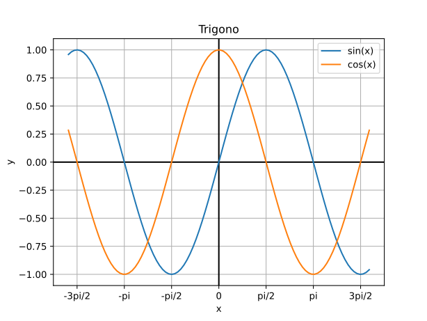
from matplotlib import pyplot as plt
import numpy as np

x = np.linspace(-5, 5, 100)
ysin = np.sin(x)
ycos = np.cos(x)
plt.figure()
plt.title("Trigono")
plt.xlabel("x")
plt.ylabel("y")
plt.grid()
plt.xticks(
  [-3*np.pi/2, -np.pi, -np.pi/2, 0, np.pi/2, np.pi, 3*np.pi/2],
  labels=["-3pi/2", "-pi", "-pi/2", "0", "pi/2", "pi", "3pi/2"]
)
plt.axhline(color="k")
plt.axvline(color="k")
plt.plot(x, ysin, label="sin(x)")     # on donne une étiquette à la courbe
plt.plot(x, ycos, label="cos(x)")     # on donne une étiquette à la courbe
plt.legend()                          # on demande d'afficher la légende
plt.show()

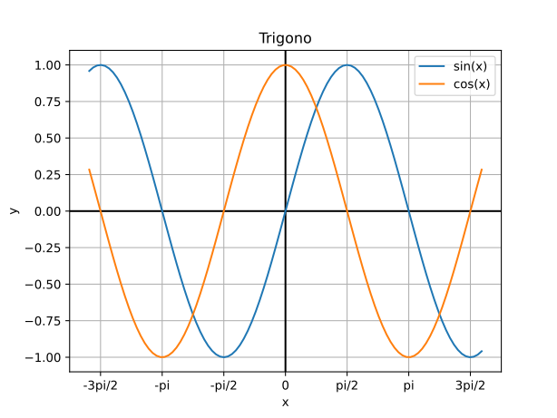
Remarque `matplotlib` deux API

Tous les exemples précédents ont été donnés dans l’API implicite de matplotlib Qui ressemble plus à Matlab
Voici un exemple dans l’API explicite:

from matplotlib import pyplot as plt
import numpy as np

x = np.linspace(-5, 5, 100)
ysin = np.sin(x)
ycos = np.cos(x)

fig, ax = plt.subplots()

ax.set_title("Trigono")
ax.set_xlabel("x")
ax.set_ylabel("y")
ax.grid()
ax.set_xticks([-3*np.pi/2, -np.pi, -np.pi/2, 0, np.pi/2, np.pi, 3*np.pi/2],
  labels=["-3pi/2", "-pi", "-pi/2", "0", "pi/2", "pi", "3pi/2"])
ax.axhline(color="k")
ax.axvline(color="k")
ax.plot(x, ysin, label="sin(x)")
ax.plot(x, ycos, label="cos(x)")
ax.legend()

plt.show()

Deux API

API implicite

plt.subplot(1, 2, 1)
plt.plot([1, 2, 3], [0, 0.5, 0.2])

plt.subplot(1, 2, 2)
plt.plot([3, 2, 1], [0, 0.5, 0.2])

plt.suptitle('Implicit Interface')

for i in range(1, 3):
  plt.subplot(1, 2, i)
  plt.xlabel('Boo')

plt.show()

API explicite

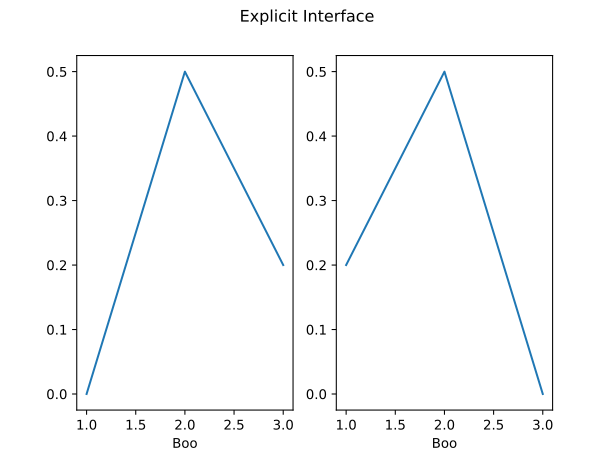
fig, axs = plt.subplots(1, 2)

axs[0].plot([1, 2, 3], [0, 0.5, 0.2])
axs[1].plot([3, 2, 1], [0, 0.5, 0.2])

fig.suptitle('Explicit Interface')

for i in range(2):
  axs[i].set_xlabel('Boo')

plt.show()

Scipy

Algorithmes et fonctions utilitaires construits sur numpy
De nombreuses fonctionnalités
- Intégration numérique
- Optimisation
- Distributions statistiques
- …
Installation

> python -m pip install scipy

Recherche de racine

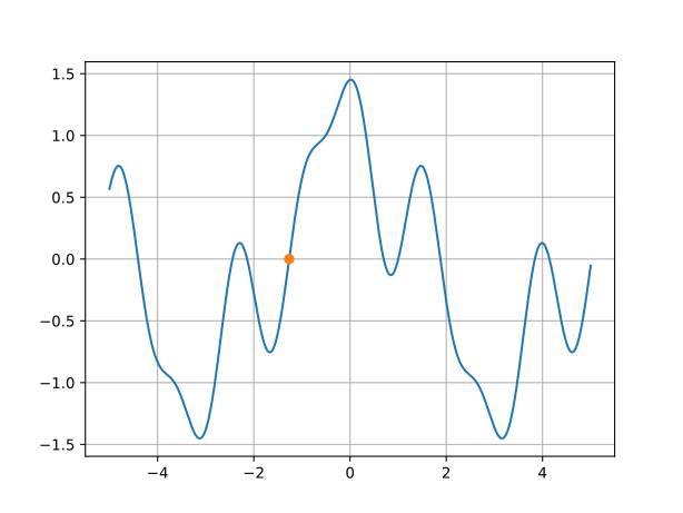
scipy intègre la recherche dichotomique vue l’année passée

from scipy import optimize

def fun(x):
  return np.cos(x)+np.cos(3*x+1)/2+np.cos(5*x-1)/3

root = optimize.bisect(fun, -2, 0, xtol=0.00001)  # xtol = 2e-12 par défaut

print(root)   # affiche -1.2646560668945312

x = np.linspace(-5, 5, 1000)
plt.figure()
plt.plot(x, fun(x))
plt.plot(root, 0, "o")  # affiche un point sur la figure
plt.grid()
plt.show()

Résultat du bisect — Résultat du `bisect`

Recherche de racine

Avec la méthode de Newton

from scipy import optimize

def fun(x):
  return np.cos(x)+np.cos(3*x+1)/2+np.cos(5*x-1)/3

root = optimize.newton(fun, -1)
print(root)  # -1.2646564339411952

Converge plus vite
Plus instable

Intégrale définie

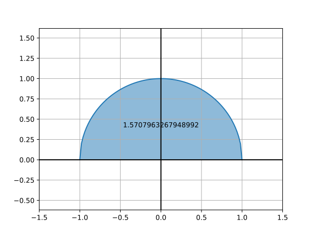
Intégration numérique avec integrate.quad

from scipy import integrate

def fun(x):
    return np.sqrt(1 - x**2)

result = integrate.quad(fun, -1, 1)
print(result)  # (pi/2, erreur)

x = np.linspace(-1, 1, 100)
y = fun(x)

plt.figure()
plt.fill_between(x, y, alpha=0.5) # colorie l'aire sous la courbe
plt.plot(x, y)
plt.grid()
plt.axis("equal")                 # même échelle sur les 2 axes
plt.xlim(-1.5, 1.5)               # limites de l'axe x
plt.axhline(color="k")
plt.axvline(color="k")
plt.annotate(str(result[0]), xy=(0, 0.4), ha="center") # ajoute un texte
plt.show()

Résultat de integrate.quad — Résultat de `integrate.quad`

Algèbre Linéaire

import numpy as np
from scipy import linalg

A = np.array([[1 , 2] , [3 , 4]])
b = np.array([[5] , [6]])
A.T            # transpose
linalg.det(A)  # déterminant
linalg.inv(A)  # inverse
A @ b          # produit matriciel

Algèbre Linéaire

Résolution de système d'équations linéaires

$\begin{cases} 1x+2y=5 \\ 3x+4y=6 \end{cases}$

$\begin{pmatrix} 1 & 2 \\ 3 & 4 \end{pmatrix} \begin{pmatrix} x \\ y \end{pmatrix} = \begin{pmatrix} 5 \\ 6 \end{pmatrix}$

$\begin{pmatrix} x \\ y \end{pmatrix} = \begin{pmatrix} 1 & 2 \\ 3 & 4 \end{pmatrix}^{-1} \begin{pmatrix} 5 \\ 6 \end{pmatrix}$

import numpy as np
from scipy import linalg

A = np.array([[1 , 2] , [3 , 4]])
b = np.array([[5] , [6]])

linalg.inv(A).dot(b)
linalg.solve(A, b)

Équations différentielles

Équation différentielle avec conditions initiales

$\frac{dy(t)}{dt} = t - y(t)$

Avec scipy

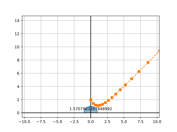
from matplotlib import pyplot as plt
from scipy.integrate import solve_ivp
import numpy as np

def fun(t: float, y: float) -> float:
  return t-y

sol = solve_ivp(
  fun=fun,
  t_span=[0, 15],
  y0=[2],
  rtol = 1e-5
)

plt.plot(sol.t, sol.y[0], '--s')
plt.show()

Équations différentielles d’ordres supérieurs

$\frac{d^2 y(t)}{dt^2} + \frac{dy(t)}{dt} + 2 y(t) = 0$

solve_ivp ne supporte que le premier ordre mais il supporte les systèmes d’équations différentielles
Nous pouvons poser que $g(t) = \frac{dy(t)}{dt}$ et réécrire l’équation sous forme d’un système du premier ordre

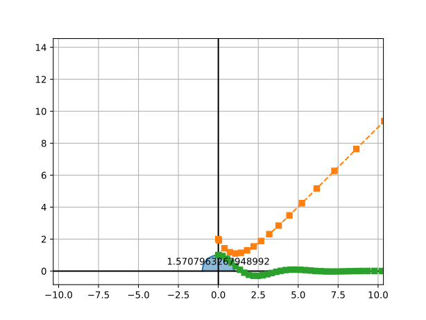
$\begin{cases} \frac{dy(t)}{dt} = g(t) \\ \frac{dg(t)}{dt} = -2 y(t) - g(t) \end{cases}$

from matplotlib import pyplot as plt
from scipy.integrate import solve_ivp
import numpy as np


def fun(t: float, Y: list[float]) -> list[float]:
  """
  Args:
    - `Y`: `Y[0]` is the value of `y(t)`
           `Y[1]` is the value of `g(t)`
    - `t`: is just the value of `t`

  Returns:
  A list with the value `y'(t)` and `g'(t)`
  """
  return [Y[1], -2*Y[0]-Y[1]]

sol = solve_ivp(
  fun=fun,
  t_span=[0, 15],
  y0=[1, 0],           # Conditions initiales pour y(t) et g(t)
  rtol = 1e-5
)

plt.plot(sol.t, sol.y[0], '--s')
plt.show()

Opérations sur des tableaux de données avec `pandas`

Manipulation de tableau de données un peu comme Excel
Basé sur numpy
Très utilisé dans le domaine des Data Sciences

> pip install pandas

Importer des données

pandas permet d’importer de multiples formats de données.

import pandas as ps

dataframe = ps.read_excel("foo.xlsx")
print(dataframe)

matricule name project labs exam 0 LUR Quentin Lurkin 15 20 20 1 LRG André Lorge 20 15 20 2 DLH Quentin Delhaye 20 20 15

Opérations sur les données

Une fois les données dans un Dataframe, il est possible de les manipuler très efficacement.

dataframe["total"] = (
  dataframe["project"] +
  dataframe["exam"] +
  dataframe["labs"]
) / 3
print(dataframe)

Cours 6 Calculs numériques

Rappels

Rappels: Calcul numérique

Outil: `numpy`

`numpy`

Vecteurs

Opérations

Fonctions vectorisées

Créer une fonction vectorisée

`numpy`: Calcul Matriciel

Même opérations que le vecteurs

Attributs

Indexation

Méthodes

Graphiques de fonctions

Créer un graphique

Style

Plusieurs courbes

Remarque `matplotlib` deux API

Deux API

API implicite

API explicite

Scipy

Recherche de racine

Recherche de racine

Intégrale définie

Algèbre Linéaire

Algèbre Linéaire

Équations différentielles

Équations différentielles d’ordres supérieurs

Opérations sur des tableaux de données avec `pandas`

Importer des données

Opérations sur les données

Exporter des données

Documentations

Rappels

Rappels: Calcul numérique

Outil: numpy

numpy

Vecteurs

Opérations

Fonctions vectorisées

Créer une fonction vectorisée

numpy: Calcul Matriciel

Même opérations que le vecteurs

Attributs

Indexation

Méthodes

Graphiques de fonctions

Créer un graphique

Style

Plusieurs courbes

Remarque matplotlib deux API

Deux API

API implicite

API explicite

Scipy

Recherche de racine

Recherche de racine

Intégrale définie

Algèbre Linéaire

Algèbre Linéaire

Équations différentielles

Équations différentielles d’ordres supérieurs

Opérations sur des tableaux de données avec pandas

Importer des données

Opérations sur les données

Exporter des données

Documentations

Outil: `numpy`

`numpy`

`numpy`: Calcul Matriciel

Remarque `matplotlib` deux API

Opérations sur des tableaux de données avec `pandas`